The tourist demand of the hotel chain. Time series for a forecast model
(*)Reinier Fernández López; (**)José Alberto Vilalta Alonso; (***)Arely Quintero Silverio; (****)Ledy Díaz González
(*)University of Pinar del Río Hermanos
Saíz Monte de Oca
Pinar del Río, Pinar del Río, Cuba
rflopez@upr.edu.cu
(**)Technological University of Havana
José Antonio Echeverría
La Habana, La Habana, Cuba
jvilalta@ind.cujae.edu.cu
(***)University of Pinar del Río Hermanos
Saíz Monte de Oca
Pinar del Río, Pinar del Río, Cuba
arelys@upr.edu.cu
(****)University of Pinar del Río Hermanos
Saíz Monte de Oca
Pinar del Río, Pinar del Río, Cuba
ledy@upr.edu.cu
Reception date: 08/12/2020 – Revision date: 10/07/2020 – Approval date: 12/15/2020
DOI: https://doi.org/10.36995/j.visiondefuturo.2021.25.01.004.en
ABSTRACT
In an increasingly uncertain world where world dynamics accelerates the way of managing processes in any sector, the forecast of tourist demand becomes very important. In this sense, the present research aims to forecast the tourist demand of the Cuban Hotel Chain of Pinar del Río, Cuba, until December 2019, through the use of time series techniques, which facilitate planning and decision-making. in this sector and in this way work towards the achievement of an integration in the productive chains, considering that tourism is one of the socioeconomic activities that activates many other sectors of production and services, as well as predicting the behavior of tourism. For this, the quantitative research method was used as the guiding method, based on the Box - Jenkins methodology and the Holt - Winters exponential smoothing method. It is also possible to characterize tourism management taking into consideration two indicators: cost per weight and average income per tourist, referring to efficiency and effectiveness respectively. In addition, a multivariate analysis of time series was carried out that made it possible to characterize the tourist activity in four fundamental stages in the hotel chain taken as the object of study.
KEY WORDS: Tourist demand; Efficacy; Efficiency; Time series.
INTRODUCTION
Tourism is one of the world's engines of development. Each year more people are on the move than ever before in history. With good planning and management, tourism can be a positive force that brings benefits to destinations around the world, but if these are deficient, it can be a factor of degradation (Hącia, 2019). It is considered one of the most diverse industries since it encompasses almost all industries in all sectors in the chain (Xie et al., 2020).
On the other hand, tourism has innumerable effects of social order, it can also be seen as an economic activity by defining elements, such as the satisfaction of needs (leisure and recreation), the expenses and expenditures that travel entails for tourists, the consumption and tourist demand, the generation of wealth, through the tourist production process, among others. That is why the tourism sector must be able to understand demand (Feng et al., 2019).
Hence the importance of studying the tourist demand of a destination, which focuses on knowing the characteristics of travelers, related to the segment to which they belong, tourist spending, the level of satisfaction of the destination's attractions, etc. It is valid to say that the analysis of the distinctive features of the tourist demand will lead to the design of actions that tend to improve the capacity of the destination to satisfy the leisure needs and desires of the tourist (Wu et al., 2017).
For this reason, demand must be forecast to plan the production system, supply and shipments, so that the supply chain operates correctly. Forecasts allow obtaining relevant, accurate and reliable information; for which companies must correctly use the most appropriate models and procedures for this purpose (C. Li et al., 2020).
At the organizational level, the demand forecast is an essential input for any decision in the different functional areas: sales, production, purchasing, finance and accounting. Forecasts are also required in supply and distribution plans. The importance of a forecast with a low margin of error is critical to efficiency and effectiveness. This has been largely recognized by various authors (S. Li et al., 2018).
Among the most relevant authors that address elements of the studies of tourism demand in Cuba are: Madrazo et al. (2009), which only proposes a procedure for the management of tourist demand and explains that estimating future demand is a challenge for scholars and planners of this activity.
Later, Barbosa and Gutiérrez (2010) suggested the application of the classic decomposition methods for the analysis of demand to know, among other elements, trend and seasonality without using advanced techniques. In a more innovative field, Gómez (2012) determines the tourist demand with artificial neural networks involving market variables, but does not include an analysis of the temporary factors that have affected tourist activity, such as the effect of economic crises.
In this sense, Castro and Fernández (2014) propose as a novelty the inclusion of the effect of climate change on tourism, that same year Cruz-Rodríguez and González-Laucirica (2014) characterize the issuing market by age group and sex, applying descriptive statistics basic form. In a more current setting, Díaz-Pompa et al. (2020) foresees a growth in tourism demand only taking into account the data of the World Tourism Organization (UNWTO) for the year 2015.
These studies propose models that consider as advantage features of the forecast of tourist demand in the short and medium term; but they do not explicitly cover the various factors that have influenced them over time. The tourist demand forecasts lack projections with different margins of error for a more in depth analysis or simply mention the tourist demand forecast as a fundamental tool for decision making without making practical use of it.
In this context, the present research aims to forecast the tourist demand of the Cubanacan Hotel Chain in the province of Pinar del Río, Cuba, until December 2019 and to characterize tourism management taking into consideration two indicators: the cost per weight and the average income per tourist, each referring to efficiency and effectiveness respectively.
DEVELOPMENT
Conceptual theoretical framework
Forecasts of tourism demand are closely related to the effective management of the destination and the timely allocation of resources, which are of continuing interest to those interested in tourism. In this sense, different authors have carried out studies that show the diversity, progress and scientific rigor of the demand forecasting tools in this strategic sector, among the first are those of Crouch (1994), who carries out an exhaustive search for the literature and where it discusses the similarities and differences in approaches for researchers who wish to conduct similar studies.
Next, Li et al. (2005) propose a study on models and forecasts of international tourism demand using econometric approaches and identify new works developed and show that the applications of advanced econometric methods improve the understanding of international tourism demand and its linkage with other sectors. In this same area, Song and Li (2008) carry out a bibliographic review and determine as key findings of this review that the methods used to analyze and forecast tourism demand have been more diverse than those identified by other authors prior to their research. Furthermore, it shows that several new techniques have emerged in the literature.
According to Song and Li (2008), when it comes to forecasting accuracy, the study shows that there is no single model that consistently outperforms other models in all situations. Additionally, this study identifies new research directions, including improving prediction accuracy by combining predictions.
In a more current context, Song et al. (2019) makes a selection of the most relevant authors in a more encompassing field that deal with issues about the forecast of tourist demand, dividing these methodologies into two large groups: time series methods and econometric methods, these associated with dynamic methods and static respectively. It also includes a new classification based on four categories: time series, econometric models, methods based on artificial intelligence and methods based on judgments.
Within these studies, it can be determined that there is little research that includes multivariate analysis of time series including indicators of efficiency and effectiveness for the analysis of tourism management. The bibliographic review shows special attention in the models to be applied. Forecasting methodologies are very diverse as researchers use both time series and econometric approaches to estimate tourism demand.
Materials and methods
Empirical research methods, based on scientific observation and documentary analysis, were used to characterize the current situation of tourist demand in Pinar del Río, Cuba.
Among the mathematical statistical methods, tools such as the Box - Jenkins methodology and the Holt - Winters exponential smoothing method were used. The software R 3.6.3 and R Studio 1.2.5033 were used to process the data and available information. Theoretical methods were also used to review the development of current tourism management processes in the province of Pinar del Río, Cuba.
Monthly data provided by Mintur were used as materials that include the number of tourists, the cost per dollar and the average income per tourist. The cost per dollar is determined by dividing the cost between the income (cost / income) while the average income per tourist is established by dividing income by the number of tourists (income / number of tourists); Both indicators are taken as indicators of efficiency and effectiveness where the lower the cost per dollar, the greater the efficiency, and the higher the average income, the greater the effectiveness. The data set covers the period between January 2006 and December 2018, for the application of the methods.
The structure selected was Cubanacan Hotel Chain, since it is the one that generates the highest income and achieves the greatest link with the rest of the productive and service sectors by having the largest presence in the territory according to the information provided by the decision makers.
Box – Jenkins Methodology
In this study, one of the statistical procedures that is implemented for the predictions is the one shown in figure 1.
The predictions begin with the identification of the Autoregressive Process of Integration of Moving Averages using the auto - aryma functions of R. The estimated parameters form the model, which is validated by analyzing the residuals. If this model is adequate, we proceed to the forecast. The residuals must be unrelated ![]() for the model to be adequate (Bakar & Rosbi, 2017). This is what is known as the Box - Jenkins methodology.
for the model to be adequate (Bakar & Rosbi, 2017). This is what is known as the Box - Jenkins methodology.

Figure No 1: Summary of the procedure for prediction statistics
Source: Bakar and Rosbi (2017)
Auto Regressive Integrated Moving Average Model
The Autoregressive Integrated Moving Average model (ARIMA) is made up of two models, the Autoregressive (AR) and the Moving Average (MA). The ARIMA model has specific parameters for the time series: the parameters p and q, which represent the order of the AR and the order of the MA, respectively. A parameter d is added that represents the number of differences (Bakar & Rosbi, 2017). Known as the Box - Jenkins (BJ) methodology, but technically known as the ARIMA methodology (Al-Musaylh et al., 2018), it ushered in a new generation of forecasting tools.
The AR model is written as: ![]() ;
; ![]() are the AR parameters, c it is a constant, p it is the order of the AR, and ut it is the white noise. The MA model can be written as:
are the AR parameters, c it is a constant, p it is the order of the AR, and ut it is the white noise. The MA model can be written as:![]() ; where
; where ![]() are the MA parameters;
are the MA parameters; ![]() are the white noise terms and u is what is expected of yt. Integrating these models, the ARIMA model is obtained, which has the following expression:
are the white noise terms and u is what is expected of yt. Integrating these models, the ARIMA model is obtained, which has the following expression: ![]() , where p and q are the terms of the autoregressive process and moving averages respectively.
, where p and q are the terms of the autoregressive process and moving averages respectively.
Seasonal Auto Regressive Integrated Moving Average Model
The Seasonal Autoregressive Integrated Moving Average model (SARIMA) is an extension of ARIMA in the event that the stationary series presents the seasonal component, which includes new terms for the 12th order differentiation (Bakar & Rosbi, 2017). The seasonal ARIMA models (P, D, Q) complement the general non seasonal ARIMA model (p, d, q), developed to capture the quarterly or semi-annual seasonal patterns present in the time series (Box et al., 1970). The combination of non-seasonal ARIMA models (p, d, q) with seasonal ARIMA (P, D, Q) leads to the SARIMA model (p, d, q) x (P, D, Q), also known as multiplicative ARIMA (Milenković et al., 2018).
In aggregate form, its general representation is: ![]() , where: d is the number of regular differences, D is the number of seasonal differences, s is the seasonal amplitude, a optimal constant, q is the number of components of moving averages, Q is the number of components of means,
, where: d is the number of regular differences, D is the number of seasonal differences, s is the seasonal amplitude, a optimal constant, q is the number of components of moving averages, Q is the number of components of means, ![]() are the coefficients of moving averages,
are the coefficients of moving averages, ![]() are the coefficients of seasonal moving averages, p is the number of autoregressive components, P is the number of seasonal autoregressive components,
are the coefficients of seasonal moving averages, p is the number of autoregressive components, P is the number of seasonal autoregressive components, ![]() are coefficients of autoregressive processes,
are coefficients of autoregressive processes, ![]() are the coefficients of seasonal autoregressive processes.
are the coefficients of seasonal autoregressive processes.
Autocorrelation function
The autocorrelation function (ACF) is a very useful tool in identifying the order of an AM model. The ACF of an AM (q) MA is canceled after the q delay, that is, ρk≈0, for k>q, then the process can be modeled through a process of moving averages of order q, MA (q) (Rahman & Ahmar, 2017). The ACF graphically represents the correlation values for time lags (Petrevska, 2017).
Given the assumption of a stationary series, where the autocorrelation function exists r(yt) = var(yt-1), it is called the partial autocorrelation function (PACF), which represents the values for a lag k and is implemented to select the order of the AR process. This PACF is built from the following expression: ![]() . Both are used for the analysis of the residuals and to check whether the model is adequate or not (Milenković et al., 2018).
. Both are used for the analysis of the residuals and to check whether the model is adequate or not (Milenković et al., 2018).
Holt-Winters exponential smoothing
In addition to the Box - Jenkins methodology, the Holt - Winters model is implemented. It incorporates a set of procedures that make up the core of the family of time series for smoothing or exponential smoothing proposed in the late 1950s (Brown, 1959; Holt, 1957; Winters, 1960).
Unlike many other techniques, the Holt - Winters model can easily adapt to changes and trends, as well as seasonal patterns. Holt-Winters is commonly used by many companies to forecast short term demand when sales data contain seasonal trends and patterns in an underlying way.
The basic structure of the Holt-Winters technique is based on the modification of the previous exponential smoothing technique, which is expanded to include a seasonal adjustment parameter. In this work, Winters smoothing is considered, which is a method of smoothing time series that present trend and seasonality, it consists of three equations, each of which updates a factor associated with each of the components of the series: randomness level, trend and seasonality.
The method uses a set of recursive estimates from the historical series. These estimates use constants; a y β and for updating the level, trend and seasonality respectively in reference to the components of the time series in question (Su et al., 2018).
There are two variations of this method: the additive method when the seasonal variations are approximately constant throughout the series, with the following component form: ![]() as a forecast equation,
as a forecast equation, ![]() as a level equation,
as a level equation, ![]() representing the trend and
representing the trend and ![]() as an equation representing the trend seasonality.
as an equation representing the trend seasonality.
The multiplicative method is applied when the seasonal variations change proportionally to the level of the series, with the following component form: ![]() forecast equation,
forecast equation, ![]() level equation,
level equation, ![]() trend equation,
trend equation, ![]() seasonality equation.
seasonality equation.
Results
In order to analyze the behavior of the tourist demand series in the Cubanacan Hotel Chain, in the period between January 2006 and December 2018, a graphic representation of it is carried out. In Figure 2, the series can be classified as stationary, since it oscillates around a mean value.
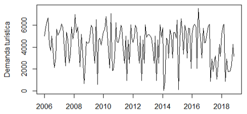
Figure No 2: Time series of monthly tourist demand (Cubanacan Hotel Chain, 2006-2018)
Source: R, version 3.6.3
When decomposing the time series for the analysis of trend and seasonality, a graph is presented containing each component of the series, obtained by means of the method of moving averages provided by the mathematical assistant R. Figure 3 shows the values observed, the seasonal component, the trend and the residuals.
It is noticeable that tourist demand tends to decrease in the last year and the strongest component is seasonality.
There are also three important fluctuations: the first begins in 2008 due to the global economic crisis and the scourge of Hurricanes Gustav and Ike; the second is evidenced as of 2013 when the world panics due to the pandemic outbreak of the Ebola disease and the third after 2015, due to the opening of Cuba-United States relations; however, showing a decrease in 2017 as a consequence of the decline in these relationships.
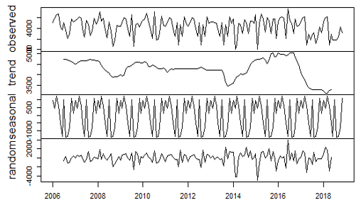
Figure No 3: Decomposition method by moving averages additive model for the tourist demand time series in Cubanacan Hotel Chain
Source: R, version 3.6.3
In the box graphs, it can be seen that the years with the highest peaks were 2006, 2007, 2013 and 2016. In 2013, the highest number of tourist visitors occurred with low variability and the decrease is corroborated as of 2017 (figure 4a).
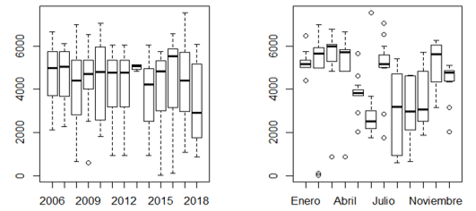
Figure No 4 (a and b): Box graphs of tourist demand by year and by month (Cubanacan Hotel Chain)
Source: R, version 3.6.3
If the series is described by months, the seasons that predominate in the hotel chain can be observed: high season and low season, corresponding to the winter and summer months. It is extracted from the graph in figure 4b that the months with the most tourism stability are January and May. This is not the case for the months from August to November as shown in table 1.
Table No 1: Average for tourist demand by years and by months

Source: Own elaboration
Previously, it was identified that the tourist demand series in Cubanacan Hotel Chain is stationary and whose strongest component is the seasonal one, as shown by the correlogram in figure 5 as it contains relative maximums with period 12.

Figure No 5: Graph of the autocorrelation function for the tourist demand time series
Cubanacan Hotel Chain
Source: R, version 3.6.3
Taking into account the characteristics of the series, Jadhav et al. (2017) and Petrevska (2017) suggest that the most recommended option is the use of the SARIMA models. It will be necessary to perform a differentiation of order 12 to eliminate seasonality and thus achieve a purely stationary series prior to applying the model.
The auto - arima function of R selects the best model automatically. This is corroborated in the work of Liu et al. (2020), the results obtained through the software are shown in table 2.
Table No 2: SARIMA models for the tourist demand time series
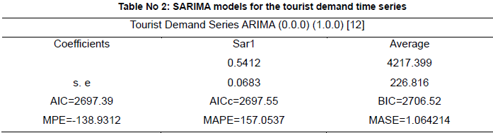
Source: Own elaboration
The most appropriate model that minimizes all measures of dispersion is a model with a twelfth-order and one-order differentiation in the autoregressive part of seasonality, that is, a SARIMA model (0, 0, 0) (1, 0, 0)
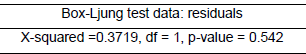
To validate the model, the Ljung-Box-Pierce test is performed, also known as the portmanteau test. The null hypothesis is that the first autocorrelations are null. The result in table 3 implies that the correlations are equal to zero and, therefore, it can be assumed that the residuals behave like white noise.
Table No 3: Ljung-Box Test

Source: Own elaboration
The graphical representation of the standardized residuals in Figure 6 shows that these vary around zero, without trend, with constant variance and there are no outliers.
Approximately 95% of the standardized residuals should be between -2 and 2 standard deviations.

Figure No 6. Graph of the standardized residuals of the SARIMA model
Source: R, version 3.6.3
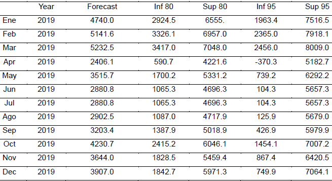
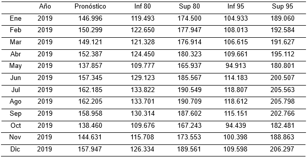
The forecast of the monthly tourist demand of the Cubanacan Hotel Chain for the year 2019 is shown in the output of R of table 4.
In this the forecast is observed through intervals for 80 and 95% confidence.
Table No 4: Forecast of tourist demand for the year 2019
Source: Own elaboration
Using the plot function of R it is possible to obtain the graphical representation of the tourist demand series, with its forecast for the next year as shown in figure 7.
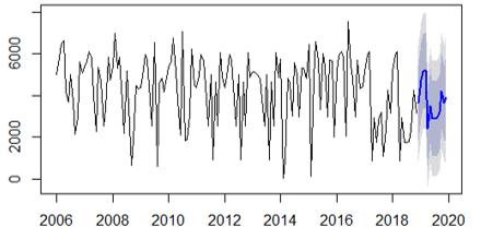
Figure No 7: Forecast of tourist demand Cubanacan Hotel Chain for the year 2019
Source: R, version 3.6.3
It is not enough only to analyze the forecast of demand in a certain sector, it is also necessary to know the behavior of its efficiency and effectiveness, in this case seen from two indicators: cost per dollar and average income per tourist to support the tourist demand series and obtain different forecasts that will help Mintur and the Cubanacan Hotel Chain to better understand what the latter's behavior is and why.
In this sense, the analysis of the Cubanacan Hotel Chain is carried out through the previously defined efficiency indicator, and the graphical representation is made for the cost per dollar series from 2006 to 2018 as shown in figure 8.

Figure No 8: Time series of the cost by monthly dollar (Cubanacan Hotel Chain, 2006-2018)
Source: R, version 3.6.3
The characteristics shown by the cost per dollar series cause the decomposition method used to be the local polynomial regression adjustment (Loess for its acronym in English).
In figure 9 it can be seen that the predominant component is seasonality.
The graph of the smoothed series (trend) shows the influence of the world economic crisis and the passage of hurricanes Gustav and Ike in 2008 with a considerable increase in cost per dollar. In 2015, there is a decrease in the series due to the occurrence of the change in policy of the United States towards Cuba, manifesting in the opposite way in 2017.
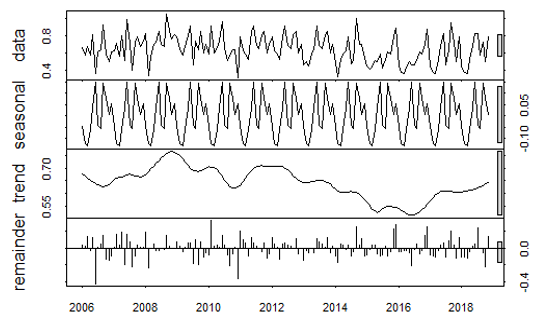
Figure No 9: Loess decomposition method additive model of the monthly cost per dollar time series
Source: R, version 3.6.3
The correlogram of the series, figure 10, allows us to verify that there is a predominance of the seasonal component, evidenced by the presence of a relative maximum for delay 12; in addition to the trend component being present, but to a lesser degree as the values of the autocorrelation function go from positive to negative.
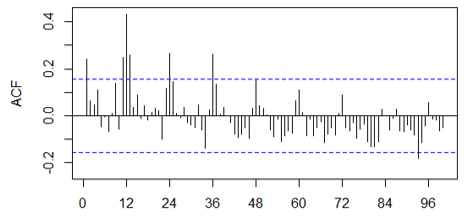
Figure No 10: Graph of the autocorrelation function of the time series cost per dollar
Source: R, version 3.6.3
Based on the characteristics of the cost per dollar series, the Holt-Winters smoothing was used as a forecasting tool, since it is used with series that present trend and seasonality. As Castillo (2017) well explains when determining that in time series with this type of characteristic, exponential smoothing minimizes the measurements referring to error. The tool depends on the alpha, beta and gamma parameters. This method provides the dispersion measures for each model obtained, being selected the one that presents the minimum values of variability as shown in table 5, obtained from the software output.
Table No 5: Holt-Winters exponential
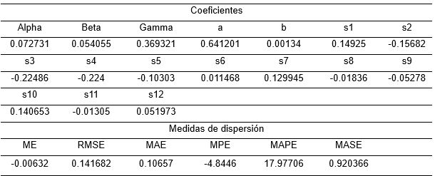
Source: Own elaboration
The model estimated by the automatic Holt-Winters function of R, which minimizes the dispersion function, is the one that comprises the parameters with values of 0.0727, 0.054 and 0.3693 for alpha, beta and gamma respectively. It is corroborated that in this model the component with the greatest weight for prediction is seasonality (gamma = 0.3693).
The quality of the model for the forecast of the cost per dollar time series is verified by analyzing the residuals through the Ljung-Box-Pierce contrast test. The application of this test allows to assert that the residuals behave as white noise as shown in table 6, according to the probability value (p value> 0.05).
Table No 6: Ljung-Box Test
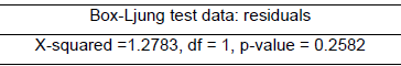
Source: Own elaboration
The graphic representation of the residuals confirms the fulfillment of the basic assumptions, this allows to affirm that the model selected for the prediction has the adequate quality as shown in figure 11.

Figure No 11: Graph of the standardized residuals of the Holt-Winters model
Source: R, version 3.6.3
From R's forecast library, the prediction for the year 2019 is formed, as well as the estimate by intervals for a reliability of 80 and 95%. The results are shown in the table below.
Table No 7: Forecast of tourist demand for the year 2019
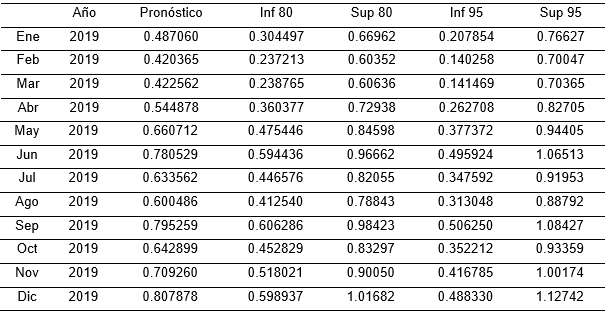
Source: Own elaboration
The graphical representation of the forecast obtained allows to visualize the probable behavior over time of the cost per dollar of the Cubanacan Hotel Chain, which is shown in figure 12.
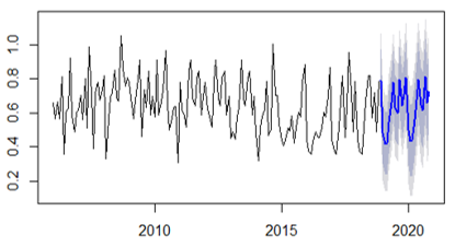
Figure No 12: Forecast of the monthly cost per dollar in the Cubanacan Hotel Chain for the year 2019
Source: R, version 3.6.3
After analyzing the tourist demand and cost per dollar series, it is necessary to analyze the efficiency indicator: average monthly income per tourist, an element of great importance for any organization. Therefore, the time series is studied below, from 2006 to 2018 represented
in figure 13.

Figure No 13: Time series of average income per tourist (Cubanacan Hotel Chain, 2006-2018)
Source: R, version 3.6.3
It starts from the decomposition of the series using the Loess method, where little influence is observed from the economic crisis that occurred in 2008 and the passage of hurricanes Gustav and Ike, contrary to what happened with the rest of the indicators studied with anteriority. There is an exponential growth in average income per tourist as of 2014, despite the tendency to decrease tourism in this hotel chain. This is due to two factors: the entry of middle and middle class tourists, that is, a more consumer tourist or tourists entering the country for the first time. In 2017, a small fluctuation was evident due to the decline in diplomatic relations between Cuba and the United States, referenced in figure 14.
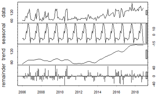
Figure No 14: Loess decomposition method additive model for the time series average income per tourist in the Cubanacan Hotel Chain
Source: R, version 3.6.3
The observation of the correlogram of figure 15 shows that the predominant component is the trend, since the autocorrelation values go from positive to negative values as illustrated in the figure; However, the seasonal component is also present as it is evident that the autocorrelations present a relative maximum with period 12.

Figure No 15: Graph of the autocorrelation function for the time series average income per tourist in the Cubanacan Hotel Chain
Source: R, version 3.6.3
The characteristics that are inherent to the average income per tourist series suggest that the most appropriate methodology in this case is exponential smoothing, in particular the Holt - Winters method, which is used in time series that present trend and seasonality, an element that has already been explained previously.
In the output of R from table 8, we have the model that best fits according to the automatic function of the software, which selects the mathematical model that contains the smallest dispersion measures from the exponential smoothing methods.
Table No 8: Holt-Winters exponential.

Source: Own elaboration
Proceeding to demonstrate the quality of the model, the Ljung-Box-Pierce contrast test shown in Table 9 is performed, which allows corroborating the behavior of the residuals as white noise (p-value> 0.05).
Table No 9: Ljung-Box Test
Source: Own elaboration
The graphic analysis of the residuals allows us to see that they behave as white noise. There is no dependency relationship between them as shown in figure 16.
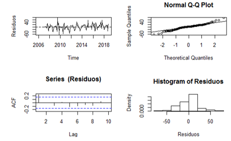
Figure No 16: Graph of the standardized residuals of the Holt - Winters prediction model
Source: R, version 3.6.3
Table 10 shows the forecast of the average income per tourist for the year 2019 in the Cubanacan Hotel Chain.
Table No 10: Forecast of tourist demand for the year 2019
Source: Own elaboration
Next, figure 17 contains the graphical representation of the predictions for the year 2019. In it, a constant variability can be observed for the forecast.
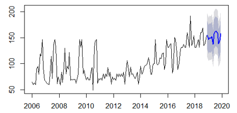
Figure No 17: Forecast of the average income per monthly tourist in the Cubanacan Hotel Chain for the year 2019
Source: R, version 3.6.3
Once the forecasting models for the efficiency and efficacy series have been presented, their multivariate analysis is continued so that it is possible to interpret how the Cubanacan Hotel Chain has behaved over time and in turn characterize it.

Figure No 18. Multivariate time series of tourism demand and the efficiency and effectiveness indicators (Cubanacan Hotel Chain, 2006-2018)
Source: R, version 3.6.3
The multivariate representation contained in figure 18 constitutes one of the graphs with the greatest explanatory power in this research.
This allows us to appreciate the relationship between the three elements taken as the object of study: tourist demand, cost per dollar and average income per tourist.
In it, the behavior of the Cubanacan Hotel Chain can be characterized in four fundamental stages: stage of deficiency in tourism management until 2008, in which there is a reduction in tourism activity and therefore the average income per tourist decreases. However, the cost per dollar increases, meaning a management deficit in the hotel chain. Stage of economic recession until 2014. This stage is identified by the negative effect caused by the world economic crisis as of 2008, also characterized by the fall in average income per tourist and a relatively constant tourist activity, on the other hand, an increase in efficiency occurs. Stage marked by the reestablishment of official relations between Cuba and the United States, in 2016, which brought as a positive effect an increase in tourist demand and a substantial increase in efficiency and effectiveness in this sector. Stage of the rupture from the year 2017, at this time the tourist demand declines significantly, but the average monthly income per tourist increases and the cost per dollar remains relatively constant, projecting an adequate effectiveness in terms of tourism management.
CONCLUSION
The demand forecast is pertinent to adequately interconnect the productive or service sectors that in one way or another intervene in the tourist activity, therefore, the mathematical models of time series have to be present for an adequate planning in this strategic economic activity and thus improve the quality of the decision making process. At this point, the study achieves the mathematical models to diagnose the tourist demand in the Cubanacan Hotel Chain in terms of its efficiency and effectiveness. A sharp drop in this sector is forecast for the coming years, aggravated by the economic situation in the country, worsening in the period of breakdown of diplomatic relations between Cuba and the United States as of 2017. To this should be added the consequences negative effects of the COVID - 19 pandemic bring for the short and medium terms. In this complex context, the need arises to combine forecasting models with the design of probable scenarios, in which these can materialize, which encourages the combination of quantitative methods with qualitative methods. Finally, the behavior of tourism management in the hotel chain is characterized over time in four stages: stage of deficiency in tourism management, stage of economic recession, stage of diplomatic relations and stage of rupture.
REFERENCES
Please refer to articles in Spanish Bibliography.
BIBLIOGRAPHICAL ABSTRACT
Please refer to articles Spanish Biographical abstract.