Prediction of transition probability from unemployment to employment in Argentina (2003-2019)

(*)Agustin Staudt; (**)Juan Luis Heredia

(*)Ministry of Productive Development of Argentina
Autonomus City of Buenos Aires, Argentina
Agusstaudt@gmail.com

(**)MisES Consulting
Autonomus City of Buenos Aires, Argentina
Juanluish012@gmail.com

Reception date: 09/19/2020 – Revision date: 12/15/2020 – Approval date: 01/11/2021
DOI: https://doi.org/10.36995/j.visiondefuturo.2021.25.02R.001.en

ABSTRACT

Despite their growing participation in the labor market, women who decide to go out and look for a job face greater difficulties in obtaining it. The participation of women in the labor force is considerably lower, even if entering the labor market the possibility of actually finding a job is also less than the chance that men have of doing so (CIPPEC, 2019). Being able to predict the probability of occupational insertion of men and women, and inquire about the factors that influence this probability, is essential in order to understand gender gaps in the labor market, helping to improve the design and implementation of public policies with a gender perspective, with the final goal to achieve equality of opportunities. In this framework, the present work will seek to predict the probability of transition from unemployment to the employment in Argentina from 2003 to 2019, using the Permanent Household Survey, based on traditional prediction techniques and Machine Learning, with the objective to find the most robust model that achieves the highest level of accuracy.

KEY WORDS: Gender; Employment; Inequality; Machine Learning.

INTRODUCTION

For the last 60 years, there has been a massive insertion of women into the labor market. This insertion is part of a deep transformation that occurred in the last century in different areas such as education, family and employment. On the one side, women's decision-making went from being static, with a limited horizon, to contemplating dynamic decisions, with long-term horizons. Furthermore, the focus of the traditional labor role becomes secondary and they begin to associate employment as a matter of identity and social value. These factors implied a change in their approach, the concept of "work" gave way to that of a "career" (Goldin, 2006).
However, gender gaps still persist: in Latin America, women participate less than men in the labor market, and if they do, they tend to work in lower-quality, part-time, underpaid jobs, and often are under-represented in the top level and decision-making posts. In fact, 95 percent of adult males between 25 and 54 years old actively work or seek employment, whereas the proportion of women falls to 66 percent (CAF 2019, Ministry of Labor 2018). In Argentina, 62 percent of women between 16 and 59 years old participate in the labor market, which represents a gap of 19 percentage points with respect to the male labor force, which is at 81 percent according to data from the Permanent Household Survey (EPH in Spanish) for the fourth quarter of 2018 (CIPPEC, 2019).
These labor inequalities emerge mainly from distortions that limit or skew decisions related to formation of human capital, family and employment during their lifetime, either due to the existence of traditional division of labor, the roles of women and man1 in the household, presence of labor discrimination or due to variables related to fluctuations in the level of economic activity (CAF 2019, CIPPEC 2019).
Although in recent years the literature has focused on studying the determinants of labor force participation of men and women, the gap in gender insertion to the labor market is a relevant problem because greater labor participation rate might not translate into a greater effective employment. According to CIPPEC (2019), in the fourth quarter of 2018, 11 percent of women aged 16 to 59 were unemployed, compared to 9 percent of men. This in turn is aggravated by the permanence in unemployment of women: using data from the EPH it is observed that of the total number of men seeking work in the first quarter of 2018, 50 percent find it in the same quarter of 2018 next year, while that percentage for women drops to 32 percent.
For all these reasons, the predictive analysis of unemployment transitions becomes relevant, with the aim of achieving a good understanding about the probability of labor insertion of women and men. This would make it possible to understand in greater depth what possibilities the unemployed have of actually finding a job in the future and, at the same time, to understand what underlying factors could be behind the differences in job opportunities between women and men. In this way, this document contributes to improving the design and implementation of public policies with a gender perspective through a predictive study of labor transitions from unemployment to employment, seeking to close gender gaps, with the purpose to achieve a greater equality between women and men2.
Although previous studies that focus the analysis on understanding the determinants of unemployment have already been carried out, through estimates of labor transitions to employment, few focus the analysis from a gender perspective. Opposite to this, in recent years in different fields of economics, the use of methods in machine learning (mostly supervised learning) has begun to intensify which seek to optimize prediction problems putting in the background the question of the unbiased estimator, allowing a trade-off between bias and variance of the estimator focusing, in turn, on obtaining good predictions out of the sample (Varian 2014, James et al. 2013, Kleingerg et al. 2015). This approach manages to fit complex and very flexible functional forms to the data without simply falling into overfitting, finding functions that, when predicting, perform well outside the sample (Mullainathan and Spiess, 2017).
Taking into account this last approach, research that seeks to predict job transitions with supervised learning methods is still scarce in our region, since they revolve around the problem of producing predictions of y from x (Mullainathan and Spiess, 2017).
In this framework, the present work investigates the characteristics of gender labor transitions from unemployment to employment through a probability prediction strategy for the Argentine labor market during the period 2003-2019, with the aim of finding the model with the highest consistency and predictive power, thus comparing the performance presented by the traditional approach and commonly used by the literature3, with respect to supervised learning.
First, a logistic regression is used to estimate the probabilities mentioned above. In order to find the best prediction, an analysis is carried out with Machine Learning classification methodologies. Given that the linear model has clear advantages in terms of inference and is often surprisingly competitive in terms of prediction in relation to non-linear methods, it could be improved by shrinking the estimated coefficients. That is, in order to improve the prediction of the model by decreasing its variance, the coefficients are contracted towards zero in relation to traditional estimates such as ordinary least squares, logit, probit, among others (James et al. 2013). For this reason the ridge and lasso regression methods are used which in the first case shrinks the coefficients asymptotically to zero, and in the second case shrinks them to zero.
This document is organized as follows. In section 2 a literature review is performed, section 3 describes the data source as well as the methodology used. Finally, section 4 presents the main results, both from the descriptive and econometric analysis.

DEVELOPMENT

Literature review

There is extensive literature that studies the transitions of individuals to different labor market states, based on their socio-demographic, institutional and macroeconomic variables, some focusing on a certain group of the population or the total of a certain country. Among the different works many differ in the estimation methodology of the transition matrix, in the functional forms or in the geographic scope of the study, be it economies at the national, regional or other level. In the case of Russell and O'Connell (2001), they analyze the transition probability of young individuals in 9 European countries, taking into account individual, socio-demographic and macro-institutional variables.
The same is done by Fabrizi and Mussida (2009), who estimate the transitions of individuals in Italy using a multinomial logit model with a Markov chain approach for the beginning and end of the decade under study. In this work, they conclude that there are fewer job opportunities for young people and women, with men having a greater probability of being employed. For the specific case of Argentina, Iturriza, Bedi, and Sparrow (2008) analyze the transition from unemployment to employment from 2002 to 2003, a period after the 2001 crisis, for individuals who received social assistance through the "Plan Jefes de Hogar". Using a logit analysis, they estimate the probability of transition in order to test the hypothesis that beneficiaries would be less incentive to seek work once they began to receive the benefit. They conclude, firstly, that the transition to employment is often delayed since the cost of being unemployed is lower. Secondly, the transition of women to employment is less than that of men, and consequently, the composition of social assistance and unemployed participants tends to be feminized. Finally, Favata (2020) not only analyzes transitions, but in his analysis also includes the study of the average duration of unemployment, finding that the age range, region, head of household and the fact of being a woman or not, can be factors that influence the possibility of remaining unemployed.

Source of Information

For this research it was used the microdata of the Permanent Household Survey (EPH in Spanish), the largest survey of socio-labor information in Argentina, carried out by the National Institute of Statistics and Censuses (INDEC). This survey is representative of the urban population of the 31 largest urban agglomerations in the country and has been carried out continuously since 2003.
This survey is carried out individually interviewing each person once during a quarter period. Additionally, there are follow-up interviews during three more quarters, alternating each period through the 2-2-2 rotation system, that is, the individual is interviewed through two quarters in succession, leaving the panel by the next two, and is surveyed again for two consecutive quarters, to finally exit the survey. Thus, a survey of the same individual is done for one and a half years (INDEC, 2003)4.
A problem that is usually found in household surveys such as the EPH is the positive attrition rate, which decreases the number of subjects surveyed during the entire interviewing period. In order to apply the prediction strategies it is required that the individual be surveyed for at least three quarters, which occurs for 61 percent of the people surveyed by the EPH (Beccaria et al., 2016).
To study labor transitions from unemployment, with the approach this work aims, different cohorts of households and people are built using the first period when each individual in a situation of unemployment is surveyed, from which their observable characteristics are used in order to construct the predictor variables. In this way, any person who was surveyed at a certain period of time is assigned to the same cohort. Additionally, it is important to know the employment situation of each interviewee in a period following the one used to construct the regressors of the estimate. Since a person is required to be surveyed at least some quarter of the following year, the last period in which the individual is followed is taken as a reference, that is, the one that occurs in the fourth period (if complete follow-up is fulfilled) or the third period (in case he leaves before full follow-up).
It should be noted that this strategy could underestimate or overestimate the transition predictions, since using values from extreme periods would not be considering what happens in intermediate periods, that is, in the quarters that the individual is surveyed, but it is not considered as information relevant, and in the quarters that the person leaves the panel. Therefore, this bias may be due to symmetric transitions during the period not considered (getting a job and being unemployed again).
For the condition of unemployment and employment, the definition of INDEC (2011) is used, which follows the regulations of the International Labor Organization. Thus, all people who have a certain specified age (10 years or more) and who have worked at least one hour during a reference time period (one week) are considered employed5.
Unemployed people consist of those who, without having a job, are available to work and have actively sought an occupation. The EPH considers as open unemployed all people aged 10 years or more who did not work in the reference week, were available and actively looked for work at some point in the last thirty days to the interview (through resumes, newspapers / internet, asking relatives or friends, etc.)6.
In order to maximize the number of available observations, a pool is built with all the labor transition panels for the years 2003-2019, identifying the cohorts to which each individual belongs, giving a total of 659,346 observations. Additionally, in order to capture adequately the probabilities of insertion of male and female workers, the sample is restricted to people between 15 and 59 years of age, totaling 398,096 observations. After that, we proceed to the identification of the unemployed at time t, resulting in 15,268 observations7.

Methodology

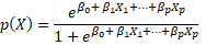
Firstly, we estimate the relationship between and X with a logistic function

From the last equation we can obtain the amount of odds,

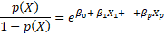
Which values can vary between zero and . Values close to zero and , show low or high likelihood of occurrence of transition from unemployment to employment respectively.
Lastly, taking logarithms on both sides of the equation we can obtain,

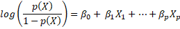
Known as log-odds or logit where an increase of X in one unit increase the log-odds in units, or equivalently in. Nonetheless, the marginal effect will depend of an specific value of X. Thus, the estimation would allow us to evaluate the effect of each regressor in the predicted variable through the sign of the coefficient, that is, a positive sign in one regressor will be associated to an increase in the variable .
To estimate the model, the maximum likelihood estimation is used, which searches for the so that the transition probability of each individual is the closest possible to the observed one. Formally, the estimated parameters are obtained by maximizing the log-likelihood function (Basto et al., 2016):

The logistic estimation is usually very useful for predictions where the dependent variable is binary, as it is in this case, in which the probabilistic limit of the estimators are equal to the parameter to be estimated. However, the estimation may have multicollinearity when variables are highly correlated, and/or the specification has many explanatory variables. In this context, the estimator is consistent but with high variance, which affects the prediction error.
Furthermore, when making predictions there is a trade-off between variance and bias. Variance refers to the amount by which the predicted data varies according to the set used as training. Regarding bias, it refers to the error that is introduced by estimating real problems with simpler statistical models. Although these components can theoretically be separated, in real life it is not possible.
Here the ridge and lasso regression estimations are useful since they shrink the coefficients by compensating a small increase in bias with a greater reduction in the variance of the prediction. Therefore, these methods handle the multicollinearity problem and show the ideal properties to minimize the numerical instability that can occur due to overfitting (Pereira, Basto and da Silva, 2016).
Thus, the ridge regression intends to maximize the following equation:

Where is the tuning parameter, which has the effect of shrinking the estimates towards zero. When the regularization or penalty term has no effect, hence the ridge estimation will produce traditional logit estimators. However, when the impact of the penalty increases, the estimated coefficients will tend to zero8. Therefore, it is key to choose an optimal value of 9.
Another alternative that is used in this document is the lasso regression which penalized version in the log-likelihood function is the following:

In the lasso estimation the tuning parameter has the effect to shrink the coefficients to exactly equal to zero, so this method performs variable selection (Basto et al. 2016; James et al. 2013)10. Finally, regarding the trade-off between variance and bias, both the ridge and lasso regressions seek to reduce an excessive variance at the expense of an increase in bias, in order to increase the precision of the prediction.
According to Pereira, Basto and da Silva (2016), the lasso regression has an advantage over ridge. Due to the possibility of selecting regressors, the final model could involve only one group of predictors, which improves its interpretability. In terms of prediction performance, the advantage that one will have over the other depends on the number of predictors that have substantial coefficients: when only a small number of predictors have coefficients of considerable magnitude, one can expect lasso to perform better, whereas when all the coefficients are approximately the same size, one expects better performance in the ridge regression.
According to Varian (2014), in order to evaluate the predictive power of each model, the results should be compared outside the sample, since when fitting a model with all the data available to the researcher, it may be that this falls into overfitting, that is, the prediction error may be underestimated. Because of this, the total dataset is divided into a training one to estimate the model, a test one to choose the model, and a validation dataset to know the performance of the chosen model. In respect to the total dataset we sample cohorts randomly for each year, being the validation dataset a total of 4268 observations. The remaining 11,000 observations are divided into one for training and one for testing, the former having 80 percent and the latter having the remaining 20 percent of the observations, both randomly chosen. Finally, it is important to clarify that on average there are 288 observations per cohort11, in addition, the average number of observations per year12 is 1018 and the average number of observations per quarter13 is 255.
In order to select the value of , a 10-fold cross validation is used, here the data is partitioned into 10 subsets of the same approximate size, in which one of the subsets is taken to be used as a test group, that is, to measure the precision of the estimated model while the remaining 9 groups are used to "train" the model, i.e., to fit the ridge and lasso regressions to these observations. This procedure is repeated 10 times, changing the test group in each one. Thus, the optimal value of lambda is the one that maximizes the cross validated log-likelihood function14. In this specific case, the optimal lambda value is sought based on the smallest binomial deviation in order to measure the error in dichotomous response variables. This is expressed as:

Where is the observed value, is the expected value, and the sum is made on the number of hits and misses, the ideal value being the binomial deviation D equal to zero.
In order to find an optimal , a vector of 101 values is first generated, starting from a value of 0 and ending in 1x1010, a set of values that is selected by the researchers’ criteria.
Finally, a measure of goodness of fit or metric is needed to compare the precision of each model when it comes to observe its predictive performance in new or unused observations in order to compute the coefficients of each regression to calculate the predicted values for the unused observations and compare them with the actual values. For this reason, the average of successes of each model is used, that is, the ratio of correct predictions over the total of observations, taking 0.5 as a cut-off point to be able to classify a predicted value as 1 (make the transition to the employment) or 0 (do not do it).

Results

Since it is a prediction exercise, the characteristics of each individual correspond to the present period (time t), while the transition to employment occurs from their future occupational status (time t +1), discarding from the analysis any future characteristics of the respondent.
In the first place, Table 1 shows the proportion unemployed in the initial period who are inserted by obtaining a job or, otherwise, continue to be unemployed.

Table N° 1: Labor Insertion

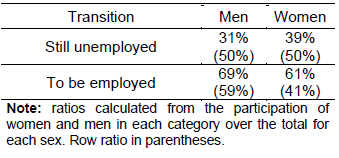
Source: own elaboration based on data from the EPH.

As can be seen from the table, of the total number of women who were unemployed in the initial period, 61 percent actually obtain a job, while the remaining 39 percent are unable to find employment in the following period. Although the distribution is similar for men, the percentage that gets a job is 8 percentage points higher than that of women15. Now, if the categories of occupational insertion between men and women are compared, it is observed that the percentage of women who manage to obtain a job is 18 percentage points less than the proportion of men.
In addition, transitions to occupation are predicted using different logit, lasso and ridge models. In the case of the estimation with logit, the results are compared with the complete data set and the test set. Then, the prediction results of the ridge and lasso models are compared with that of logit. In the logit regression, we included socio-demographic variables such as sex, age, educational level, marital status, socio-labor status such as number of registered employees and the previous occupation of the unemployed, fixed effects by region (dummies for the NEA, NOA, Cuyo, Pampeana, Patagonia and CABA-CBA) and year (2003-2018).
After this, the prediction power of the model is measured for transitions to employment or non-transition, for both men and women. The results are in the following table:

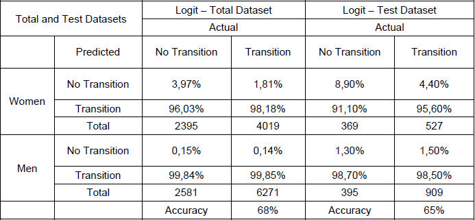
Table N° 2 confusion matrix logit regression with total and test datasets.

Source: own elaboration based on data from the EPH

In the table above, the total columns were calculated, given that the main point here is to analyze the predictive accuracy of the model for the different transition states.

On the one hand, analyzing the logit model with the total dataset, of the total number of women who obtained employment 98.18 percent of the observations were predicted correctly. On the other hand, of the total observed of women who did not transited to employment, only 4 percent were predicted correctly, the prediction percentage being much lower for non-transitions in relation to transitions. The same is true for the estimated transitions for men in which the prediction hits were 99.85 percent for transitions and an estimate of 0.15 percent for non-transitions.
Furthermore, the ridge regression is estimated including 162 variables available to estimate the transition of individuals, which includes the variables used in the logit regression and other variables related to the time searching for a job and job search method, economic sector in which the individual works, income decile, occupational category16, size of the establishment in which they worked, reasons for leaving their job, other sources of income, characteristics of the dwelling, age range, presence of children under 10 years of age and number of people in the home. The following are the results of the cross-validation:

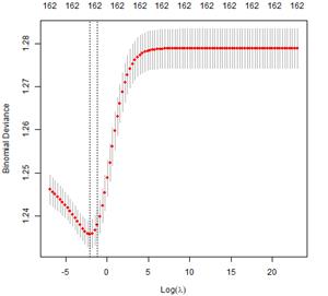
$Descripción: C:\Users\USUARIO\Google Drive\Investigacion CDNG\Investigacion Genero (mi Pc)\Borradores\Ridge_optimo.png$
Figure N° 1: Binomial deviance for different values of of ridge regression.
Source: own elaboration based on data from the EPH.

Figure N°1 shows the binomial deviation as a function of the logarithm of λ, and in the upper part is the number of variables for each lambda17.

From the different values of the regularization parameter, the minimum is found to be λ = 0.12618 (log 0.12618 = -2.07). Once the value of the tuning parameter has been obtained, the prediction error in the test base is estimated using the regressors obtained with the training base and using the optimal lambda. The results are detailed below:

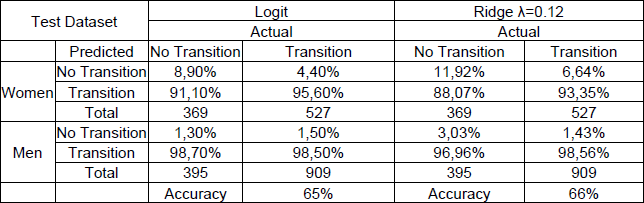
Table N° 3: Confusion matrix of logit and ridge regressions.

Fuente: own elaboration based on data from the EPH.

In the table above, the differences in prediction errors for both transition and non-transition are less than 2 percent for their respective quadrants for men and women.

As well as this, differences in the percentages of correct predictions can be noted between the ridge and logit estimates. It can be seen that in table 3 the non-transition quadrant for women has a lower percentage (8.9 percent) of correct predictions in relation to the non-transition quadrant of the ridge regression (11.92 percent). Additionally, the same happens with men since the percentage of correct predictions of the logit model in the test dataset is 1.3 percent, being lower than that of ridge (3.03 percent). In contrast to the aforementioned, the percentage of successes of the logit regression is slightly lower for men with 98.50 percent, compared to that of ridge (98.56 percent). In the case of women, the logit model has a better performance in predicting transitions with 95.6 percent correct predictions compared to the ridge estimate (93.35 percent).
As mentioned previously, the ridge tuning parameter shrinks all coefficients asymptotically towards zero (unless ), which should not cause problems to see the precision in the model prediction. However, it can create a challenge in interpreting the coefficients, in fact 162 regressors are counted in the model. Therefore, the lasso alternative could be useful, since its tuning parameter has the effect of forcing a group of estimated coefficients towards exactly zero. In this way, lasso regression also develops a selection of variables, not only penalizes them (it is a sparse model). The results of the lasso regression can be seen in the following graph:

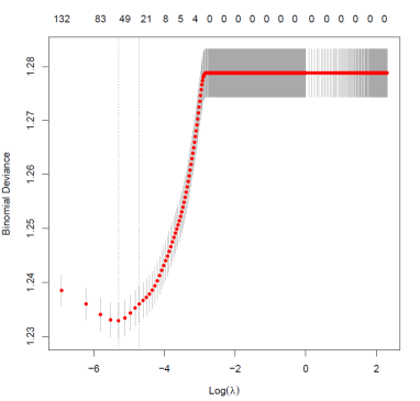
Figure N° 2: Binomial deviance for different values of in lasso regression.
Source: own elaboration based on data from the EPH.

When looking at the figure from the right to the left, it is observed that the performance improves. This is because for very large values of λ the number of variables becomes zero, while after certain values of the parameter, the model selects at least one variable and the predictive fit improves, which suggests greater gains in accuracy for values close to zero of our λ grid. In contrast, the form of the binomial deviation as a function of the logarithm of lambda is U-shaped, with a minimum for a positive value of λ. This suggests that, from the existence of a positive tuning parameter, an improvement could be found in the prediction of the labor transition under study.
The following table shows the results with lasso estimation:

Table N° 4: Confusion matrix of logit and lasso estimations in test dataset.

Source: own elaboration based on data from the EPH.

The above table shows the predictive performance of the lasso model with the value equal to 0.05.

As can be seen, this value is low but different from zero, which would suggest an improvement over the logit model. In order to prove this, it is compared with the results of the logit model used in the previous section. What can be shown is a very low improvement compared to the logistic model, reflected to a greater extent by the precision gained in lasso to predict those men and women who did not move to the employment status or remain unemployed in the following period. That being said, it is hard to make predictions in groups where the number of observations is considerably smaller, as is the case of the non-transition group versus the transition group.
One of the advantages of lasso over ridge is that the former can select variables, using only those that are relevant to make the prediction. Therefore, out of 162 variables, the lasso estimator selected 64 variables, that is, it selected less than half of the total predictors. Among the selected variables are the variables of time in which the person was looking for work, which suggest that the longer the person was looking for a job, the less likely they are to going to be employed in the following year. Furthermore, the longer the time that has elapsed since the previous occupation ended, the lower the probability to be employed in the next period.
In the case of women, the way in which they look for a job offers them different probabilities of finding it in the following year: those women who show up at establishments, send resumes, or sign up on job fairs, work lists, employment plans, etc. are less likely to be employed in the next period than the alternative of networking or interviews. Searching independently, understood as the possibility of doing something to undertake on your own, entails a greater probability of getting a job compared to searching through contacts or interviews.
On the side of the marital situation, married men or men in a domestic partnership are more likely to be employed in the following year, while married women are less likely to get a job in the following period. This could be due to the considerable search intensity of married men compared to single men, which generates this result, while the difficulties explained before in the female job search are also reflected here. Regarding the head of the household, the chances of being employed in the next period increases, regardless of gender.
So far, the traditional model, the ridge and lasso supervised learning models have been compared using a cross-validation approach, where each model was trained and its performance was compared outside the sample, through the construction of a training group in which we run each regression (80 percent of the total dataset) and a test dataset (20 percent of the dataset), where it was evaluated how well each estimator performs with out-of-sample observations through the comparison of the percentage of correctly predicted employment status with respect to the actual value. The training and testing approach proposes the random separation of a group of observations in order not to be used until the moment of checking the predictive power of the estimators outside the sample. However, the training and testing randomization process could not be totally separated from the training group, so before starting the tests an additional validation group was separated, which is made up of a randomly selected cohort per year. In other words, the same group of people who entered the survey for the first time is taken for each year, representing approximately 25 percent of the total dataset. The idea behind this strategy is to evaluate the estimators for entire groups that have not been in the data set before, seeking to reproduce performance of prediction of the estimators for new observations.

Table N° 5: Confusion Matrix of logit and ridge estimations on validation dataset.

Source: own elaboration based on data from the EPH.

Tables N° 5 and 6 show that the percentage of correctly predicted transitions of each model is approximately equal, being 71 percent for logit and 70 percent for ridge and lasso.

Although the total correct predictions of each model are similar, there are differences between each one of them. In the case of the ridge model, the percentage of correct predictions of the transitions and non-transitions is higher than that of the logit model for men.

Table N ° 6: Confusion matrix of lasso estimation on validation dataset.

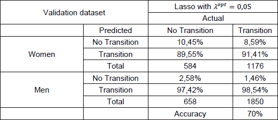
Source: own elaboration based on data from the EPH.

In the case of women, an improvement can only be seen in the prediction of non-transition. Regarding the estimation of the lasso model, the percentage of non-transition correct predictions is higher than that of the logit model in the case of men and women, but the percentage of non-transition correct predictions is lower for both genders. Therefore, it can be said that the ridge and lasso models have greater predictive power of non-transitions in relation to the logit model. Even so, it is noted that the low percentage of success in the prediction in the ridge and lasso models may be due to the low number of people who remained unemployed, some functional form that has not been tested, or the lack of some group of variables in the model.

CONCLUSION

Although there have been great progress in terms of gender, the gap between men and women is a problem that continues today. The participation of women in the labor force is considerably lower, even entering the labor market the possibility of actually finding a job is lower than men have. In fact, in the first quarter of 2018, 50 percent of men found a job in the same quarter of the following year, while that percentage for women dropped to 32 percent.
The interest in finding answers to the different unemployment transitions faced by men and women, together with the possibility of accessing other prediction tools, led us to wonder if these estimators could be more accurate in predicting labor transitions from unemployment to employment for women and men in the Argentine labor market, so as to make a more accurate characterization of the most important determinants that could predict labor insertion in a two-year period.
From the different models evaluated in this work, the percentage of correctly predicted values was calculated as a measure of goodness of fit, finding that the predictive capacity of the lasso and ridge models were better in the non-transitions, although the difference with the logit model in points percentage is low, the latter standing out for being the model with the fewest number of variables.
Regarding the coefficients of the estimates, the logit estimation had coefficients with the expected signs, specifically the dummy variable "woman", in which the probability of finding employment in the following period is lower for women than for men.
Moreover, from the lasso regression it was found that the probability of moving from the unemployment to employment decreases for married women in relation to single women, but increases for men, which could reflect the presence of traditional roles within a household, that have an impact on heterogeneous job search intensities in favor of men.
In fact, the lasso estimation suggests that the longer the time searching for a new job, the lower the probability of finding a job in the following period, likewise, the longer the time elapsed since an unemployed person finished their last job, the probability of getting a job next year decreases. The different ways a woman searches for a job also influences her probability of insertion, having greater probabilities of finding a job searching through contacts or interviews, than conducting the search by sending resumes or registering in job fairs, or employment plans, while they have a greater chance of being employed the following year if they seek it independently, that is, starting their own business.

NOTES

1.Childcare has a fundamental impact on the possibilities of women's access to the labor market (CIPPEC, 2019).

2.We are aware that part of the population does not identify with traditional genders (male and female) and at present there is no generalized consensus on the best way to classify gender. However, the information available for analysis in this document does not have a different classification. Therefore, we use the traditional division for this research.

3.There are multiplicities of methodological approaches to analyze labor market transitions. In this document we refer to a traditional approach such as the estimation through a binary logistic regression, which is common in this type of research (Freeman and Ballen 1986; Russell and O'Connell 2001; Mussida and Fabrizi 2009; Kütük and Güloglu 2019; Cerruti 2000; among others).

4.The percentage of people entering the EPH is 25 percent of the total of households surveyed in a quarter, that is, in each quarter 25 percent of households are renewed and simultaneously 25 percent of households leave the survey.

5.This includes people who in a given period worked for at least one hour, whether or not they have been paid; and people who have an occupation, but were not working for a period of time and maintained a formal link with their employer.

6.INDEC (2011) does not consider within this concept other forms of inappropriate employment such as people who carry out temporary jobs while actively looking for work, those who involuntarily work hours below average, those employed in positions below minimum pay, nor to the unemployed who have suspended their search for lack of visible job opportunities, etc.

7.It is clarified that, due to how the dataset is built by cohorts using the method explained above, there are observations that have no follow-up over time, such is the case of the cohorts that enter the 2nd quarter of 2013, 3rd and 4th of 2014 and all of 2015.

8. However, the tuning parameter will not shrink them to exactly zero.

9.It should be clarified that the estimated coefficients are not scale invariant in these models, since will not only depend on the lambda values, but also on the scale of the predictors. So these are standardized:

10. It should be clarified that we want to reduce the estimated association of each variable with the outcome. However, we do not want to reduce the intercept, which is simply a measure of the mean value of the response when all regressors are exactly zero.

11.The total number of cohorts under analysis is 62.

12. The total number of years under analysis is 19.

13. The period covered begins in the first quarter of 2003 ending in the third quarter of 2018. Additionally, it is clarified that there is no information on the third quarter of 2007, second quarter of 2013, third and fourth of 2014, all of 2015 and the first quarter of 2016. In the case of the years 2007, 2013, 2015 and 2016, it was due to the interruption in the publication of the EPH. In the case of 2014, it was due to the lack of follow-up in the following year, of the individuals who entered the cohort in the third and fourth quarter of 2014.

14. To make the estimates we used the R software, while to estimate the ridge and lasso regressions we used the glmnet package (Friedman et al., 2020). The package allows to fit generalized linear models with different shrinkage penalties in ridge and lasso estimations.

15. Cabe destacar que no contemplamos en el trabajo la posibilidad de que los varones y mujeres desempleadas pasen a la inactividad, lo cual es una problemática igual de grave y que afecta mayormente a las mujeres (CIPPEC, 2019).

16. It refers to the unemployed with a previous occupation.

17.As the ridge method does not contract the estimators to exactly zero, for each value of lambda all variables have values greater than zero. In this case there are 162 variables.

REFERENCES

Please refer to articles in Spanish Bibliography.

BIBLIOGRAPHICAL ABSTRACT

Please refer to articles Spanish Biographical abstract.